
Complexity
Explore changing patterns, compare order with chaos, and turn complexity into a visual control.
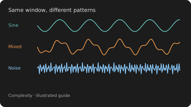
Three different experiments: watch measurements change, compare different dynamics, then use an output to animate a visual. The analysis nodes are the real Complexity bundle nodes; the included helpers provide signals and displays.
Start here
Enable Complexity and Signal. Every patch opens in one Explore tab with its graph, live display, and controls together.
The practice sources update at 10 Hz and supply 512-sample windows at 256 Hz. These are generated experiments, not live recordings. Measurement histories show recent updates.
Open the first recipe ↓ Bundle setup →
Meet the nodes
Use the node pictures to find the inputs and outputs. Each experiment points to a recipe you can build on.
Count new patterns in a sequence
Try it. Compare the rhythm, bursts, and noise in recipe 01; watch the history rather than one number.
Good to know
The node first converts samples into high and low values. The result describes that binary sequence and depends on window length.
Inputs: data: ARRAY
Outputs: complexity: ARRAY
Compare the order of nearby samples
Try it. Compare the three conditions in recipe 02, then change the logistic-map parameter.
Good to know
Order and delay choose the patterns being counted. Keep both fixed when comparing conditions.
Inputs: data: ARRAY
Outputs: entropy: ARRAY
Measure how often patterns keep matching
Try it. Add this node to ComplexityStream in recipe 01 and compare its output while keeping window length and settings fixed.
Good to know
Short or highly repetitive windows can give unstable or non-finite values. approximate switches to a different measure, approximate entropy.
Inputs: data: ARRAY
Outputs: entropy: ARRAY
Compare concentrated and spread-out power
Try it. In recipe 03, increase noise and watch the entropy-driven visual change.
Good to know
The input is a waveform with sample-rate metadata, not a PSD. Normalization and spectral method affect comparisons.
Inputs: data: ARRAY
Outputs: entropy: ARRAY
Explore the structure in a signal's recent history
Try it. Add this node to ComplexityStream in recipe 01 and compare its output while keeping window length and settings fixed.
Good to know
Order and delay define the embedding. Changing them changes the question you ask of the same signal.
Inputs: data: ARRAY
Outputs: entropy: ARRAY
Describe how quickly a trace changes
Try it. Add this node to ComplexityStream in recipe 01 and compare its output while keeping window length and settings fixed.
Good to know
A smooth sine can change faster without becoming a more irregular waveform. Read the two outputs separately.
Inputs: data: ARRAY
Outputs: mobility: ARRAY · complexity: ARRAY
Count sign changes
Try it. Add this node to ComplexityStream in recipe 01 and compare its output while keeping window length and settings fixed.
Good to know
Normalization gives crossings per sample, not per second. A DC offset or added noise can change the count.
Inputs: data: ARRAY
Outputs: count: ARRAY
Compare the roughness of traces
Try it. Add this node to ComplexityStream in recipe 01 and compare its output while keeping window length and settings fixed.
Good to know
These are different estimators. Keep the estimator, window size, and Higuchi kmax fixed for a comparison.
Inputs: data: ARRAY
Outputs: dimension: ARRAY
Explore fluctuations across time scales
Try it. Add this node to ComplexityStream in recipe 01 and compare its output while keeping window length and settings fixed.
Good to know
A fitted exponent needs a suitable range of scales. A number from a short periodic trace is not evidence of long-range memory.
Inputs: data: ARRAY
Outputs: exponent: ARRAY
Compare roughness across scales
Try it. Add this node to ComplexityStream in recipe 01 and compare its output while keeping window length and settings fixed.
Good to know
c2 near zero and negative c2 describe different scaling behaviour, but a finite-window estimate alone does not establish multifractality. Image mode reads the last two axes as a field.
Inputs: data: ARRAY
Outputs: c1: ARRAY · c2: ARRAY
Patch recipes
From regular to unpredictable
Move between a repeating rhythm, noise, and short bursts. Watch how two measurements respond over time.
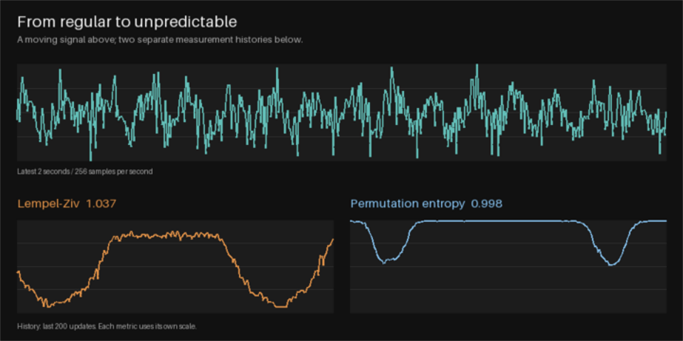
- Start with Automatic enabled and watch a full cycle from rhythm to noise.
- Turn Automatic off to set Noise yourself.
- Increase Bursts and compare both histories with the signal above.
ComplexityStream.outLempelZiv.dataComplexityStream.outPermutationEntropy.dataComplexityStream.outComplexityScope.signalLempelZiv.complexityComplexityScope.firstPermutationEntropy.entropyComplexityScope.secondWhat to look for. Lempel-Ziv counts new binary patterns; permutation entropy measures the ordering of nearby samples. Their responses need not match.
Set Noise to zero, then raise Bursts. Compare that with adding continuous noise.
Each measurement uses the latest 512 samples. Histories retain 200 updates, and use separate fixed scales. Automatic mode overrides the Noise control until you turn it off.
Order, chaos, and noise
Compare a periodic wave, a logistic map, and random noise side by side. A jagged trace can still contain a clear rule.
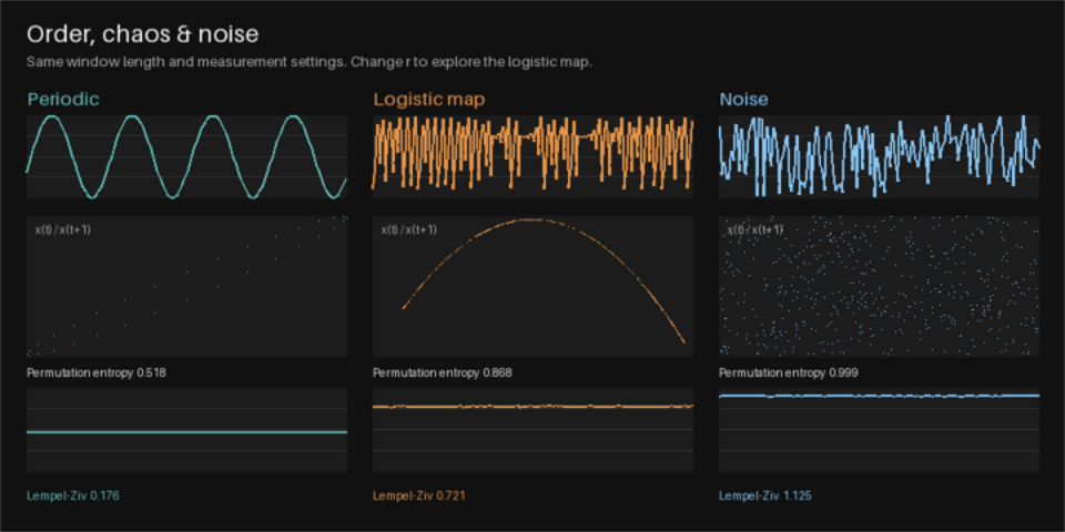
- Compare the three time traces and the lag plots beneath them.
- Change LogisticR from 3.2 to 3.5, 3.9, and 4.0.
- Watch the logistic map move between repeating and chaotic behavior, alongside the unchanged reference conditions.
DynamicsLab.outPermutationEntropy.dataDynamicsLab.outLempelZiv.dataDynamicsLab.outComplexityScope.signalPermutationEntropy.entropyComplexityScope.firstLempelZiv.complexityComplexityScope.secondWhat to look for. The logistic map follows a deterministic rule. Its lag plot has structure even when its time trace looks irregular; random noise fills a cloud.
Look for periodic windows near r = 3.83. Compare the entropy history before and after the change.
Every condition has the same 512-sample length and analysis settings. A lag plot places each sample against its next sample. Entropy alone cannot prove that a signal is chaotic.
Let complexity shape a visual
Use spectral entropy as a live control signal. Watch a smooth form become more irregular as power spreads across frequencies.
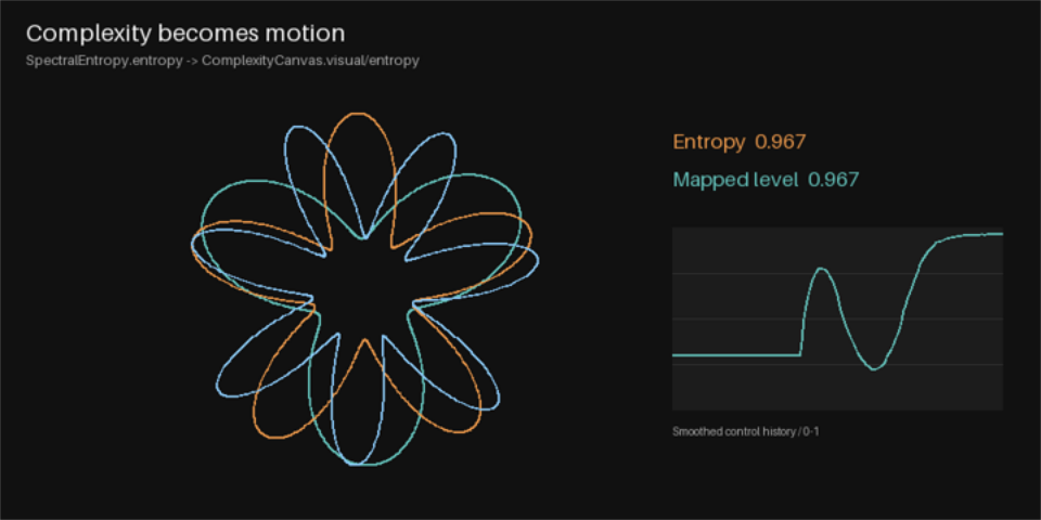
- Watch the signal and the visual together while Automatic cycles the noise amount.
- Select ComplexityCanvas and inspect visual/entropy: its reference is SpectralEntropy.entropy.
- Adjust Gain to change the response, then Smoothing to make transitions slower or more immediate.
ComplexityStream.outSpectralEntropy.dataWhat to look for. The SpectralEntropy output drives a parameter on ComplexityCanvas. The graph wire carries the waveform into the analysis; the parameter reference carries the result into the visual.
Turn Automatic off. Move Noise from 0 to 1, then compare Smoothing at 0.05 and 0.5.
The mapping clips entropy × gain to 0–1, then smooths it per update. Smoothing is a response coefficient, not seconds. The animation is an artistic mapping of spectral entropy.
Working practice
Compare like with like
Keep the sample rate, window length, preprocessing, and estimator settings the same. Change one source property, then compare each output against its own baseline.
Check the waveform first
Flat data, missing samples, drift, and clipping can dominate these measurements. Inspect the input before interpreting the number. For a live stream, place a Buffer before the analysis nodes.