
Patching
A patch is the graph plus the workspace it was saved with. A .gfi is a zip holding both.
An LSL stream, filtered, its spectrum viewed, and a FOOOF fit off the same spectrum. Every node here is one goofi ships.
Sub-patches
Grouping nodes makes a sub-patch, and it talks to the patch around it through boundary ports. A sub-patch is saved and undone like any other part of the patch.
Patching basics
Five short experiments to learn how signals move through a patch.
Download an example and follow along, or build it using the connection guide. Each screenshot shows a running patch. Click it to enlarge the nodes and their plots.
To see a node’s output, expand the output row and choose line in the viewer menu. Use the cog to adjust the plot.
For experiments with a particular bundle, explore the Cookbooks.
01 · Collect samples into a window
LFO produces a repeating wave. Buffer keeps a recent stretch of that wave so you can see several cycles at once.
- Connect LFO’s
outto Buffer’sinput. - On LFO, set
output/modetoblock,output/sfreqto 250, andlfo/frequencyto 1. This produces 250 samples per second, with one wave cycle each second. - On Buffer, set
buffer/unittosamplesandbuffer/sizeto 1000. Leavebuffer/axisat −1. - Open Buffer’s line viewer. Once the buffer fills, you should see four cycles: 1000 samples ÷ 250 samples per second = four seconds.
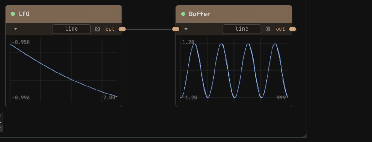
Connection guide
Change Buffer’s size to 500. You now keep two seconds of signal, so only two cycles fit in the plot. Change it back to 1000 for the next example.
Use a buffer with an EEG recording →
02 · Send one signal to several analyses
One output can connect to several inputs. Here, three analysis nodes receive the same samples from Buffer.
Add LempelZiv, SpectralEntropy, and Hjorth to the previous patch. Connect Buffer’s out to the data input on each one, then open their output viewers.
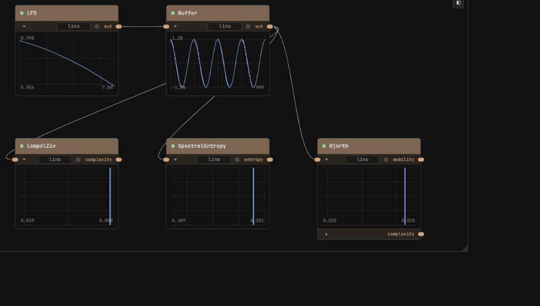
Connection guide
- LempelZiv measures how complex the signal’s patterns are.
- SpectralEntropy measures how widely its power is spread across frequencies.
- Hjorth measures how the signal changes over time, through its mobility and complexity outputs.
These outputs are single measurements. Their line viewers show the current value; they do not accumulate a history.
Change LFO’s waveform from sine to square. Watch which measurements change, then switch back. Compare each measurement with its own earlier value: the three nodes use different scales.
Use the same branching idea with EEG →
03 · Make a sound
Osc creates a tone. Filter changes its brightness, and Gain controls its volume.
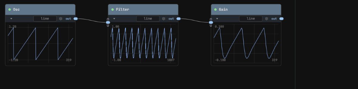
- Connect Osc → Filter → Gain, using
outandinputat each step. - Set Gain’s
gain/gainto 0. - Add AudioOut and connect Gain’s
outto itsinput. AudioOut starts audio processing and sends the sound to your device. Add it when opening any of the audio downloads on this page. - Choose a sawtooth waveform on Osc and lowpass mode on Filter. Slowly raise Gain to a comfortable listening level.
Connection guide, including AudioOut
Lower Filter’s filter/cutoff. The sound becomes less bright as the higher frequencies are reduced. Raise it again and listen to them return.
Pitch and cutoff use an octave scale: adding 1 doubles the frequency. A setting of 1 does not mean 1 Hz.
Combine tuning, sound, and visuals →
04 · See the frequencies in a sound
A waveform shows how a signal changes over time. A spectrum shows which frequencies it contains. Psd calculates a spectrum from a window of samples.
- Keep the audio chain from lesson 03 running. Draw another cable from Osc’s
outto a Buffer’sinput. - Set Buffer’s
buffer/unittosamples, its size to 8192, and its axis to −1. - Connect Buffer’s
outto Psd’sinput. Set Psd’spsd/modetofftand open its line viewer.
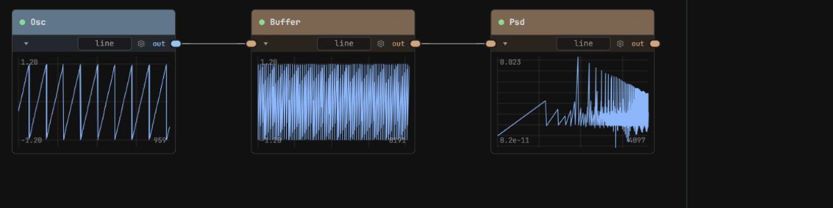
Connection guide
Switch Osc from sawtooth to sine while keeping the pitch fixed. A sine concentrates its power near one frequency. Switch back to sawtooth to see the extra peaks at multiples of that frequency.
Measure power in frequency bands →
05 · Control a parameter with a signal
Make the sound’s volume rise and fall automatically. LFO will supply a changing value for Gain’s gain parameter. This connection is called a reference, and you set it in the parameter controls.
- Add an LFO to the audio patch. Set
output/modetovalueso it sends one number at a time. - Set its frequency to 0.2, amplitude to 0.1, and offset to 0.15. This gives a value that moves between 0.05 and 0.25 over five seconds.
- Select Gain. In its parameter panel, open the
gaingroup and expand thegainfield. - Choose R · Reference, then select LFO as the node and out as the output.
Gain now follows LFO.out. Watch the gain value move in the parameter panel and listen to the volume rise and fall. Keep the audio cables from Osc through Filter and Gain to AudioOut.
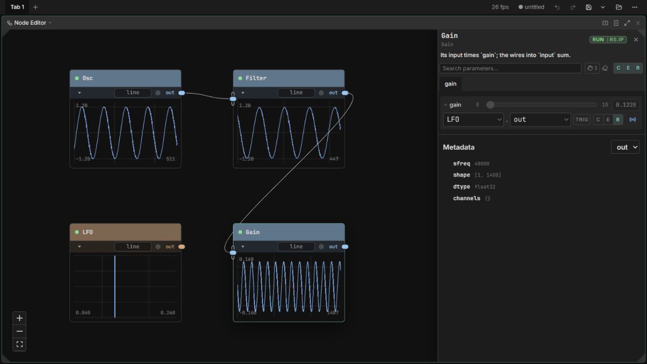
Enlarge the parameter controls ↗
Explore the parameter controls
- output / mode
- value
- frequency
- 0.2 Hz
- amplitude
- 0.1
- offset
- 0.15
Move the cycle slider to see Gain follow LFO’s output.
The arrow shows which output controls the parameter. This interactive illustration is silent; try the downloaded patch to hear the result.
Raise LFO’s frequency from 0.2 to 0.4. The volume now rises and falls twice as fast. Lower its amplitude to make the changes gentler.
The three buttons choose where a parameter gets its value:
- C · Constant: enter a fixed value. Choose this and set gain to 0.1 to stop following the LFO.
- E · Expression: calculate a value, such as
0.1 * 2. - R · Reference: follow another node’s output, as in this example.